Parkinson’s Telemonitoring

Author

Chenxi Lin

Published

July 28, 2025

About this site

Introduction

This dataset is composed of a range of biomedical voice measurements from 42 people with early-stage Parkinson’s disease recruited to a six-month trial of a telemonitoring device for remote symptom progression monitoring. The dataset includes various acoustic features such as average vocal fundamental frequency, jitter, shimmer, and harmonic-to-noise ratio, as well as two clinical outcome scores: motor UPDRS (Unified Parkinson’s Disease Rating Scale) and total UPDRS, which are standardized measures used to assess the severity and progression of Parkinson’s symptoms. The primary goal of this analysis is to investigate how voice features relate to disease severity and to develop predictive models that estimate UPDRS scores based on these vocal biomarkers.

Data source

The dataset was created by Athanasios Tsanas (tsanasthanasis@gmail.com) and Max Little (littlem@physics.ox.ac.uk) of the University of Oxford, in collaboration with 10 medical centers in the US and Intel Corporation who developed the telemonitoring device to record the speech signals. The original study used a range of linear and nonlinear regression methods to predict the clinician’s Parkinson’s disease symptom score on the UPDRS scale.

http://archive.ics.uci.edu/ml/datasets/Parkinsons+Telemonitoring

Reference

A Tsanas, MA Little, PE McSharry, LO Ramig (2009)‘Accurate telemonitoring of Parkinson’s disease progression by non-invasive speech tests’, IEEE Transactions on Biomedical

Load the packages

library(tidyverse)
library(tidymodels)
library(knitr)
library(GGally)

Load dataset

data <- read.csv("Parkinsons-Telemonitoring-ucirvine.csv")

# Turn the character "false"/"true" into a factor with labels
data <- data %>% mutate(gender = factor(sex, levels = c("false", "true"), labels = c("Female", "Male") ))

1. Exploratory Data Analysis (EDA)

1.1 Summary statistics

summary(data)

    subject           age           sex              test_time      
 Min.   : 1.00   Min.   :36.0   Length:5875        Min.   : -4.263  
 1st Qu.:10.00   1st Qu.:58.0   Class :character   1st Qu.: 46.847  
 Median :22.00   Median :65.0   Mode  :character   Median : 91.523  
 Mean   :21.49   Mean   :64.8                      Mean   : 92.864  
 3rd Qu.:33.00   3rd Qu.:72.0                      3rd Qu.:138.445  
 Max.   :42.00   Max.   :85.0                      Max.   :215.490  
  motor_updrs      total_updrs        jitter           jitter_abs       
 Min.   : 5.038   Min.   : 7.00   Min.   :0.000830   Min.   :2.250e-06  
 1st Qu.:15.000   1st Qu.:21.37   1st Qu.:0.003580   1st Qu.:2.244e-05  
 Median :20.871   Median :27.58   Median :0.004900   Median :3.453e-05  
 Mean   :21.296   Mean   :29.02   Mean   :0.006154   Mean   :4.403e-05  
 3rd Qu.:27.596   3rd Qu.:36.40   3rd Qu.:0.006800   3rd Qu.:5.333e-05  
 Max.   :39.511   Max.   :54.99   Max.   :0.099990   Max.   :4.456e-04  
   jitter_rap        jitter_ppq5         jitter_ddp          shimmer       
 Min.   :0.000330   Min.   :0.000430   Min.   :0.000980   Min.   :0.00306  
 1st Qu.:0.001580   1st Qu.:0.001820   1st Qu.:0.004730   1st Qu.:0.01912  
 Median :0.002250   Median :0.002490   Median :0.006750   Median :0.02751  
 Mean   :0.002987   Mean   :0.003277   Mean   :0.008962   Mean   :0.03404  
 3rd Qu.:0.003290   3rd Qu.:0.003460   3rd Qu.:0.009870   3rd Qu.:0.03975  
 Max.   :0.057540   Max.   :0.069560   Max.   :0.172630   Max.   :0.26863  
   shimmer_db     shimmer_apq3      shimmer_apq5     shimmer_apq11    
 Min.   :0.026   Min.   :0.00161   Min.   :0.00194   Min.   :0.00249  
 1st Qu.:0.175   1st Qu.:0.00928   1st Qu.:0.01079   1st Qu.:0.01566  
 Median :0.253   Median :0.01370   Median :0.01594   Median :0.02271  
 Mean   :0.311   Mean   :0.01716   Mean   :0.02014   Mean   :0.02748  
 3rd Qu.:0.365   3rd Qu.:0.02057   3rd Qu.:0.02375   3rd Qu.:0.03272  
 Max.   :2.107   Max.   :0.16267   Max.   :0.16702   Max.   :0.27546  
  shimmer_dda           nhr                hnr              rpde       
 Min.   :0.00484   Min.   :0.000286   Min.   : 1.659   Min.   :0.1510  
 1st Qu.:0.02783   1st Qu.:0.010955   1st Qu.:19.406   1st Qu.:0.4698  
 Median :0.04111   Median :0.018448   Median :21.920   Median :0.5423  
 Mean   :0.05147   Mean   :0.032120   Mean   :21.679   Mean   :0.5415  
 3rd Qu.:0.06173   3rd Qu.:0.031463   3rd Qu.:24.444   3rd Qu.:0.6140  
 Max.   :0.48802   Max.   :0.748260   Max.   :37.875   Max.   :0.9661  
      dfa              ppe             gender    
 Min.   :0.5140   Min.   :0.02198   Female:4008  
 1st Qu.:0.5962   1st Qu.:0.15634   Male  :1867  
 Median :0.6436   Median :0.20550                
 Mean   :0.6532   Mean   :0.21959                
 3rd Qu.:0.7113   3rd Qu.:0.26449                
 Max.   :0.8656   Max.   :0.73173

1.1.1 Summarize by group

# Compute count, mean & SD of key variables by gender
summary_by_gender <- data %>%
  group_by(gender) %>%
  summarise(
    n                  = n(),                                # sample size
    age_mean           = mean(age,           na.rm = TRUE),  # average age
    age_sd             = sd(age,             na.rm = TRUE),  # age SD
    total_updrs_mean   = mean(total_updrs,   na.rm = TRUE),  # avg total UPDRS
    total_updrs_sd     = sd(total_updrs,     na.rm = TRUE),  # SD total UPDRS
    motor_updrs_mean   = mean(motor_updrs,   na.rm = TRUE),  # avg motor UPDRS
    motor_updrs_sd     = sd(motor_updrs,     na.rm = TRUE)   
    )

# Render the summary_by_gender as a markdown table
summary_by_gender %>% kable(caption = "Table 1. Summary Statistics of Age and UPDRS by Gender")

Table 1. Summary Statistics of Age and UPDRS by Gender
gender	n	age_mean	age_sd	total_updrs_mean	total_updrs_sd	motor_updrs_mean	motor_updrs_sd
Female	4008	65.05539	7.84549	29.72406	11.004499	21.46935	7.891659
Male	1867	64.26727	10.60045	27.50523	9.849771	20.92458	8.607728

1.2 Visualize distributions & outliers of total UPDRS

1.2.1 Histogram of total UPDRS

ggplot(data, aes(x = total_updrs)) +
  geom_histogram(binwidth = 1, fill = "darkslategray3", color = "black") +
  labs(title = "Distribution of Total UPDRS", x = "Total UPDRS", y = "Count") +
  theme(axis.title.x = element_text(size = 16), 
        axis.title.y = element_text(size = 16),  
        axis.text.x  = element_text(size = 12),  
        axis.text.y  = element_text(size = 12),  
        legend.position = "none")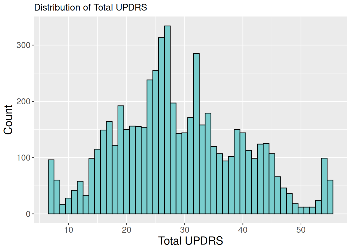

1.2.2 Density plot of total UPDRS by gender

ggplot(data, aes(x = total_updrs, fill = gender)) +
  geom_density(alpha = 0.4) +
  labs(
    title = "Density of Total UPDRS by Gender",
    x     = "Total UPDRS",
    y     = "Density")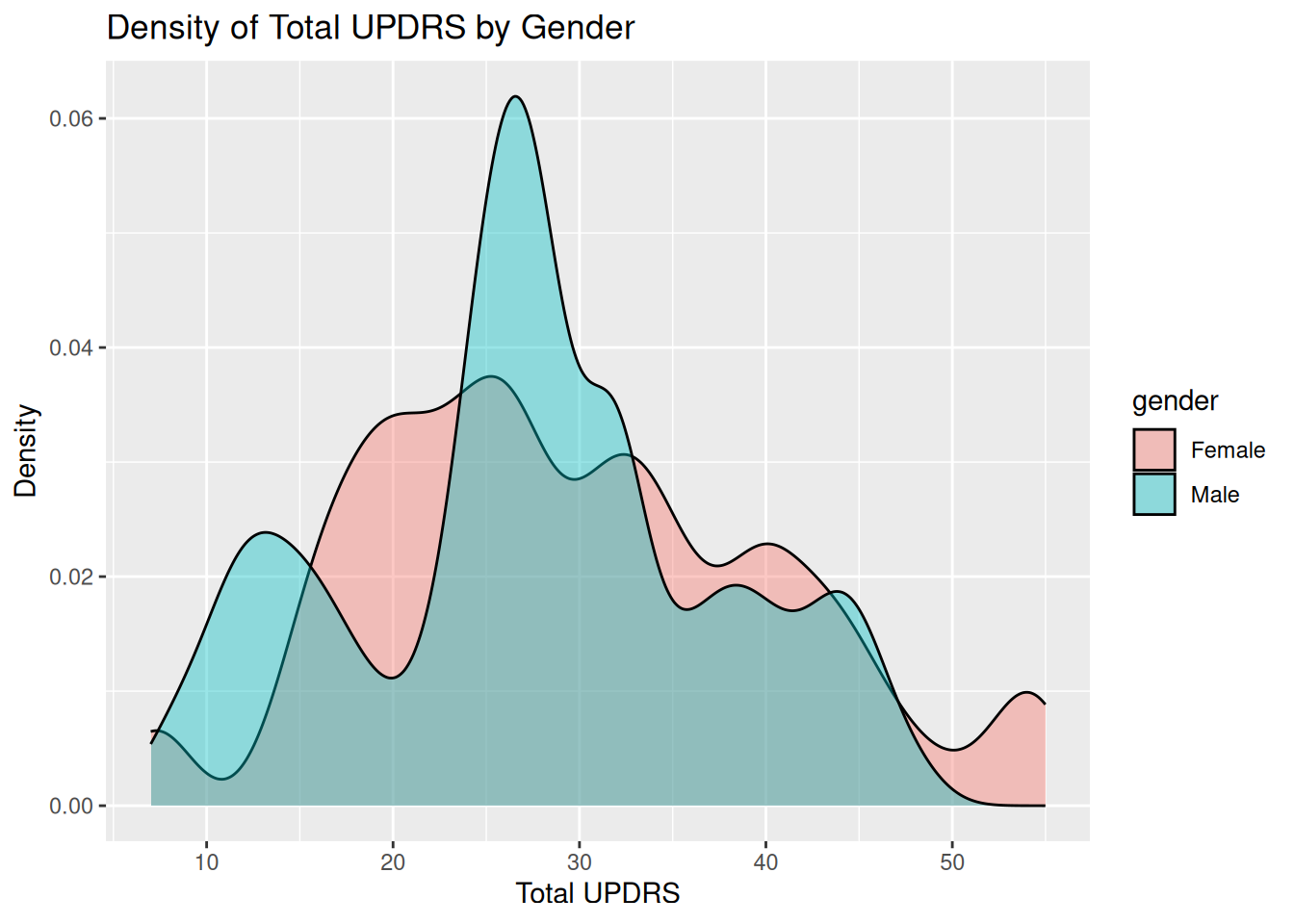

1.2.3 Violin & boxplot of motor UPDRS by gender

ggplot(data, aes(x = gender, y = motor_updrs, fill = gender)) +
  geom_violin(trim = FALSE, color = "black") +
  geom_boxplot(width = 0.1, outlier.shape = NA,
               color = "black", size = 1.2) +
  scale_fill_manual(values = c("Female" = "rosybrown2", "Male" = "darkslategray3")) +
  labs( title = "Motor UPDRS Distribution by Gender",
    x = "Gender",
    y = "Motor UPDRS") +
  theme(axis.title.x = element_text(size = 16),  
        axis.title.y = element_text(size = 16),   
        axis.text.x  = element_text(size = 12),     
        axis.text.y  = element_text(size = 12),  
        legend.position = "none")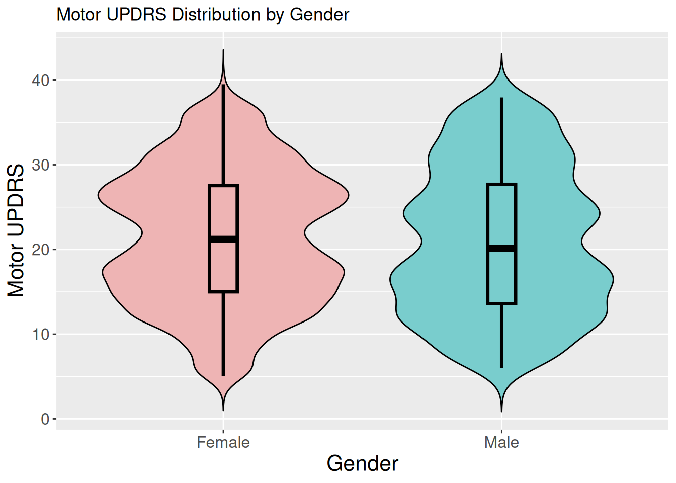

1.3 Boxplot for age vs. total UPDRS

ggplot(data, aes(x=factor(age), y=total_updrs)) +
  geom_boxplot(fill='lightgreen') +
  labs(title='Age vs. Total UPDRS', x='Age', y='Total UPDRS') +
  theme(axis.text.x = element_text(angle=0), )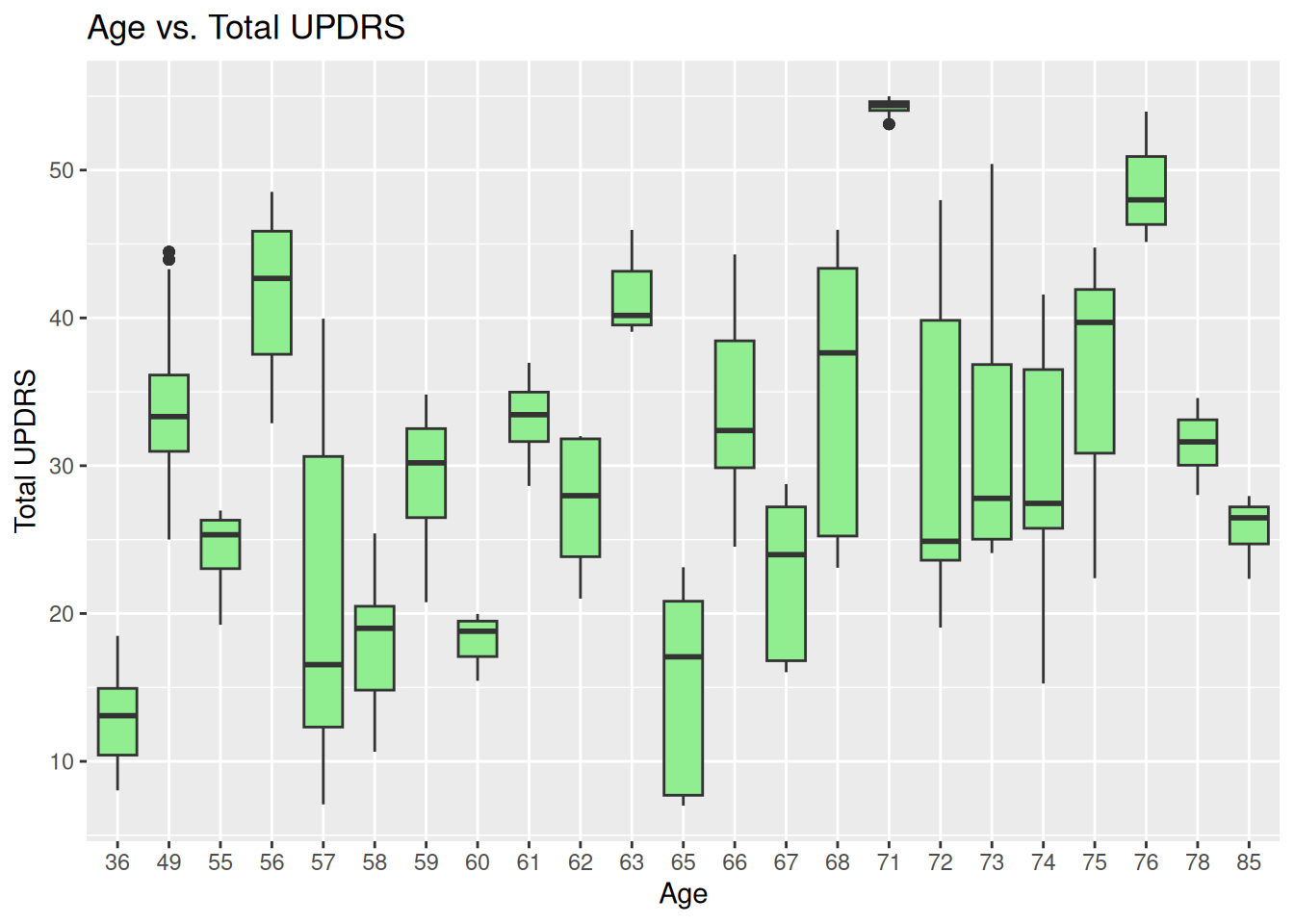

1.4 Scatterplot matrix of key measures

data %>%
  select(motor_updrs, total_updrs, jitter, shimmer, nhr, hnr) %>%
  ggpairs(title = "Pairwise Scatterplots of Vocal Measures")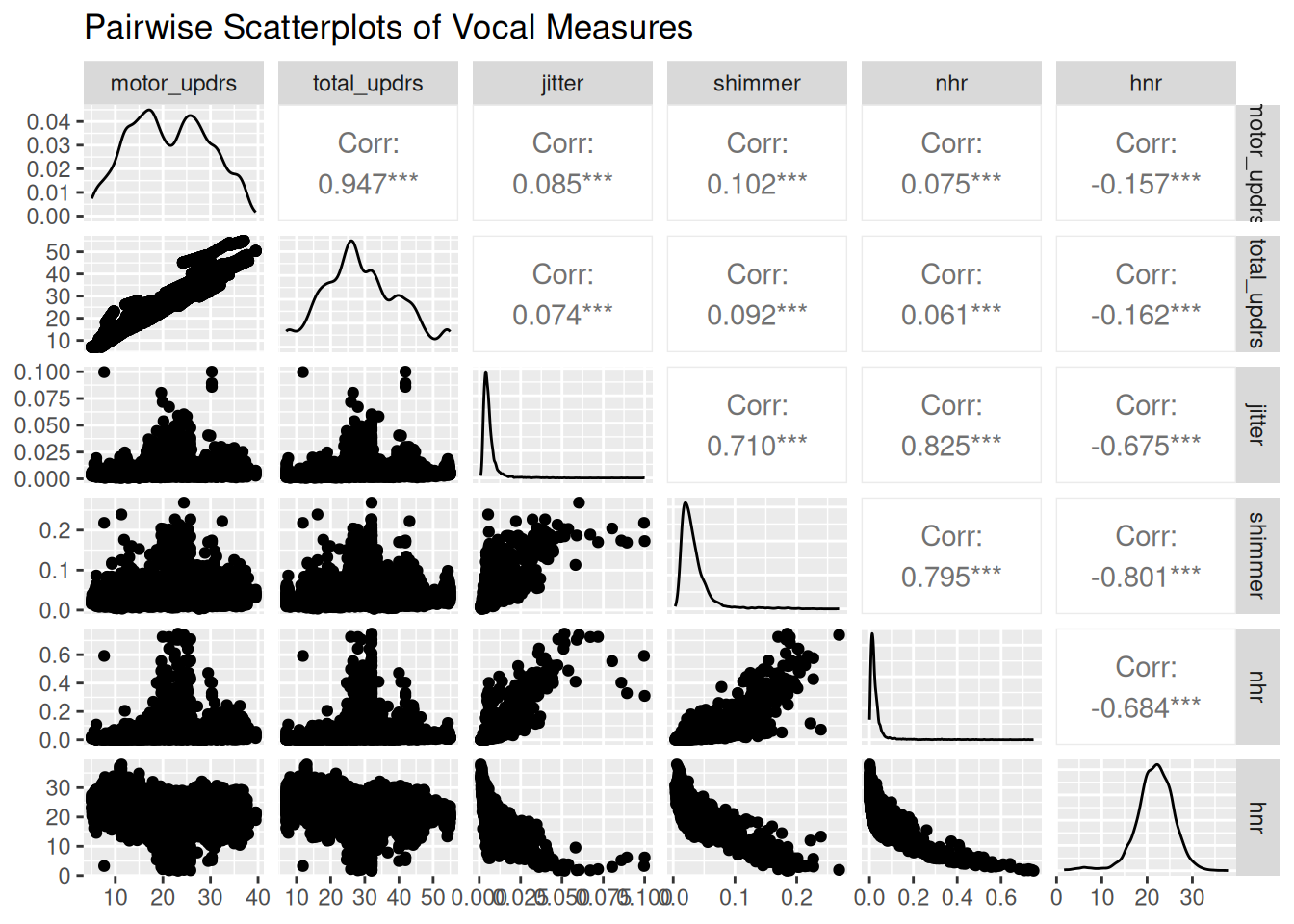

2. Correlation and Regression Analysis

2.1 Correlation matrix

num_vars <- data %>%
  select(age, motor_updrs, total_updrs, jitter, shimmer, nhr, hnr)
corr_mat <- cor(num_vars, use = "pairwise.complete.obs")

library(ggcorrplot)

ggcorrplot(
  corr_mat,
  hc.order   = TRUE,      # cluster vars
  type       = "lower",   # lower triangle
  lab        = TRUE,      # show values
  lab_size   = 3,         
  tl.cex     = 12,        # axis‐label size
  tl.srt     = 45,        # rotate labels
  tl.col     = "black",   # label colour
  outline.col= "gray70",  
  colors      = c("red", "white", "steelblue"),
  ggtheme    = theme_minimal(base_size = 14)) +
  labs(title    = "Correlogram") +
  theme(axis.text = element_text(color = "black"))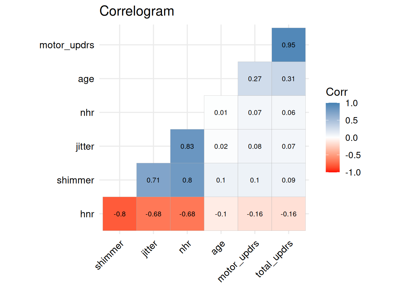

2.2 Simple linear regression

lm1 <- lm(total_updrs ~ jitter + shimmer, data = data)
summary(lm1)


Call:
lm(formula = total_updrs ~ jitter + shimmer, data = data)

Residuals:
    Min      1Q  Median      3Q     Max 
-26.365  -7.332  -1.519   7.553  26.337 

Coefficients:
            Estimate Std. Error t value Pr(>|t|)    
(Intercept)  27.6897     0.2321 119.312  < 2e-16 ***
jitter       33.9171    35.0935   0.966    0.334    
shimmer      32.9216     7.6397   4.309 1.66e-05 ***
---
Signif. codes:  0 '***' 0.001 '**' 0.01 '*' 0.05 '.' 0.1 ' ' 1

Residual standard error: 10.66 on 5872 degrees of freedom
Multiple R-squared:  0.008648,  Adjusted R-squared:  0.00831 
F-statistic: 25.61 on 2 and 5872 DF,  p-value: 8.424e-12

2.3 Multiple regression including age & gender

lm2 <- lm(total_updrs ~ jitter + shimmer + age + gender, data = data)
summary(lm2)


Call:
lm(formula = total_updrs ~ jitter + shimmer + age + gender, data = data)

Residuals:
    Min      1Q  Median      3Q     Max 
-24.449  -7.660  -1.337   7.464  24.782 

Coefficients:
            Estimate Std. Error t value Pr(>|t|)    
(Intercept)  4.88057    0.99302   4.915 9.12e-07 ***
jitter      94.01670   33.36093   2.818  0.00485 ** 
shimmer     13.07136    7.30299   1.790  0.07353 .  
age          0.36664    0.01508  24.319  < 2e-16 ***
genderMale  -2.03085    0.28395  -7.152 9.59e-13 ***
---
Signif. codes:  0 '***' 0.001 '**' 0.01 '*' 0.05 '.' 0.1 ' ' 1

Residual standard error: 10.1 on 5870 degrees of freedom
Multiple R-squared:  0.1089,    Adjusted R-squared:  0.1083 
F-statistic: 179.3 on 4 and 5870 DF,  p-value: < 2.2e-16

3. Logistic Regression

# Categorize UPDRS severity (example: mild < 20, moderate = 20-30, severe > 30)
data$severity <- cut(data$total_updrs, breaks=c(-Inf, 20, 30, Inf), labels=c("Mild", "Moderate", "Severe"))

# Logistic regression predicting severe vs non-severe
data$severe_binary <- ifelse(data$severity=="Severe", 1, 0)

# Fit logistic regression
logit_model <- glm(severe_binary ~ jitter + shimmer + age + sex, data=data, family=binomial())
summary(logit_model)


Call:
glm(formula = severe_binary ~ jitter + shimmer + age + sex, family = binomial(), 
    data = data)

Coefficients:
             Estimate Std. Error z value Pr(>|z|)    
(Intercept) -2.324343   0.209643 -11.087  < 2e-16 ***
jitter      -0.772055   6.723934  -0.115    0.909    
shimmer      6.773637   1.481060   4.574 4.80e-06 ***
age          0.029939   0.003166   9.456  < 2e-16 ***
sextrue     -0.407588   0.058676  -6.946 3.75e-12 ***
---
Signif. codes:  0 '***' 0.001 '**' 0.01 '*' 0.05 '.' 0.1 ' ' 1

(Dispersion parameter for binomial family taken to be 1)

    Null deviance: 8033.3  on 5874  degrees of freedom
Residual deviance: 7839.7  on 5870  degrees of freedom
AIC: 7849.7

Number of Fisher Scoring iterations: 4

# ROC Curve analysis
library(pROC)

Type 'citation("pROC")' for a citation.


Attaching package: 'pROC'

The following objects are masked from 'package:stats':

    cov, smooth, var

roc_obj <- roc(data$severe_binary, fitted(logit_model))

Setting levels: control = 0, case = 1

Setting direction: controls < cases

plot(roc_obj, col="darkslategray3", main="ROC Curve for Severe UPDRS Classification")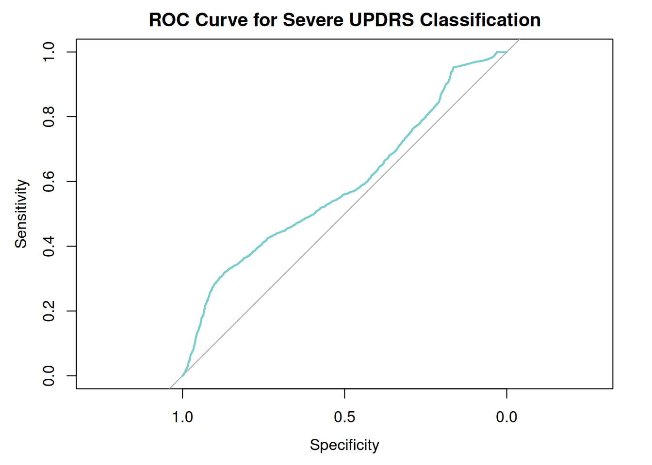

auc(roc_obj) # Area Under the Curve

Area under the curve: 0.5892

4. Cluster Analysis

# Normalize features
library(scales)
data_scaled <- data %>%
  select(jitter, shimmer, nhr, hnr) %>%
  mutate_all(rescale)

# k-means clustering (k=3 example)
set.seed(123)
kmeans_model <- kmeans(data_scaled, centers=3, nstart=25)

# Append clusters to original data
data$cluster <- factor(kmeans_model$cluster)

# Visualize clusters (using PCA for plotting)
pca_res <- prcomp(data_scaled, scale=TRUE)
pca_data <- data.frame(pca_res$x, cluster=data$cluster)

ggplot(pca_data, aes(PC1, PC2, color=cluster)) +
  geom_point(alpha=0.6) +
  labs(title="K-means Clustering (k=3)", x="PC1", y="PC2") +
  theme_minimal()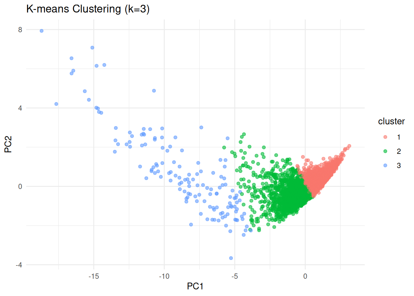

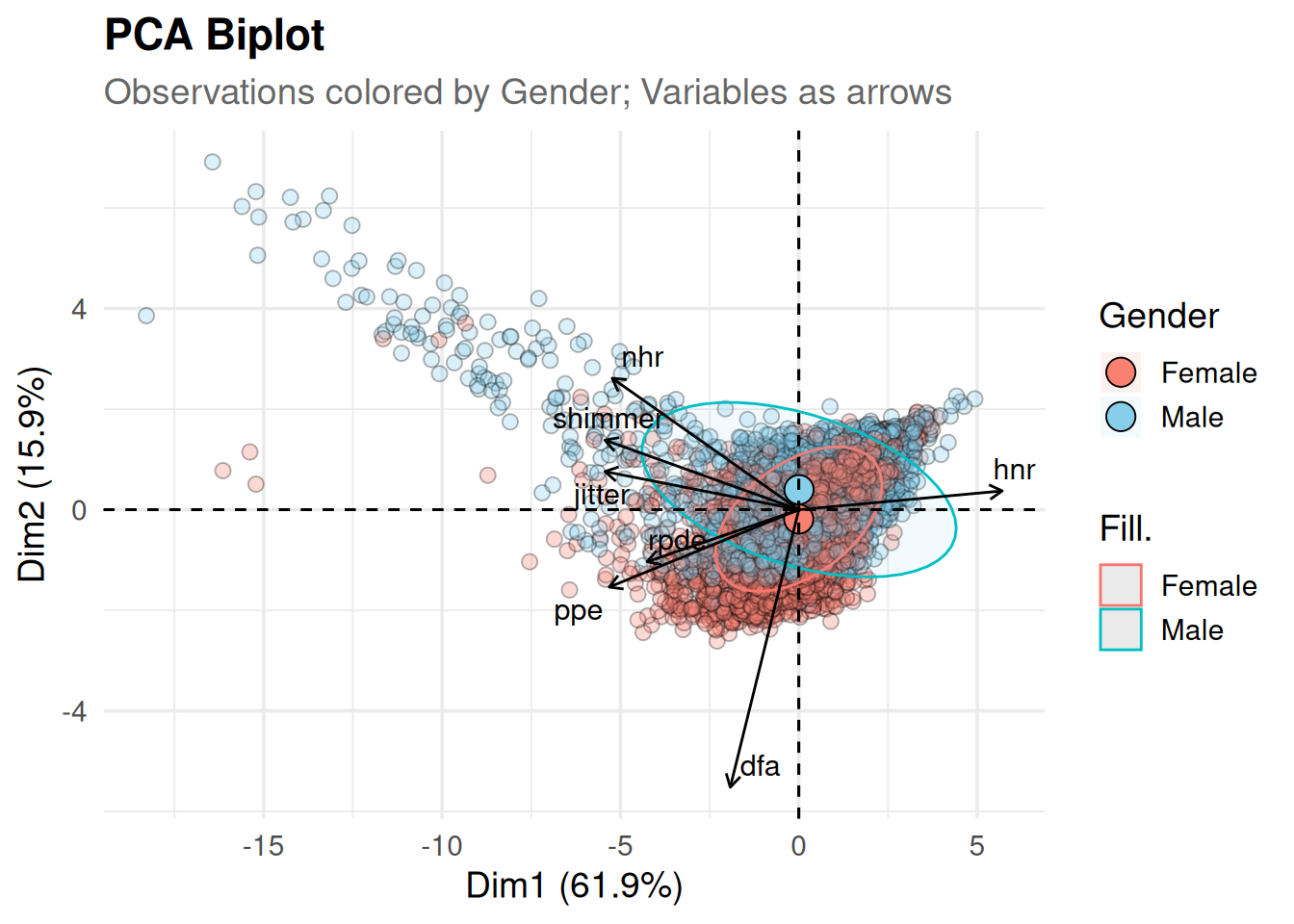
5. Principal Component Analysis (PCA)

# PCA on selected numeric variables
pca <- prcomp(data[, c("jitter", "shimmer", "nhr", "hnr", "rpde", "dfa", "ppe")], scale=TRUE)

# Summary of PCA
summary(pca)

Importance of components:
                         PC1    PC2     PC3     PC4     PC5     PC6     PC7
Standard deviation     2.082 1.0544 0.82576 0.59845 0.53083 0.36138 0.32092
Proportion of Variance 0.619 0.1588 0.09741 0.05116 0.04025 0.01866 0.01471
Cumulative Proportion  0.619 0.7778 0.87521 0.92638 0.96663 0.98529 1.00000

# Scree plot to visualize variance explained
library(factoextra)

Welcome! Want to learn more? See two factoextra-related books at https://goo.gl/ve3WBa

fviz_eig(
  pca,
  addlabels   = TRUE,              # show percent values on bars
  ylim        = c(0, 70),          # y‐axis limits (adjust as needed)
  barfill     = "steelblue",       # fill color for bars
  barcolor    = "black",           # border color
  linecolor   = "firebrick",       # color of cumulative line
  pointshape  = 19,                # shape of points on cumulative line
  pointsize   = 3,                 # size of those points
  labelsize   = 8                # size of the percent‐labels
) +
  labs(
    title = "Scree Plot",
    subtitle = "Principal components ordered by descending variance",
    x     = "Principal Component",
    y     = "Percentage of Variance"
  ) +
  theme_minimal(base_size = 14) +
  theme(
    plot.title  = element_text(face = "bold"),
    plot.subtitle  = element_text(color = "gray0"),
    panel.grid  = element_blank(), 
    axis.text.x  = element_text(size = 12), 
    axis.text.y  = element_text(size = 12) )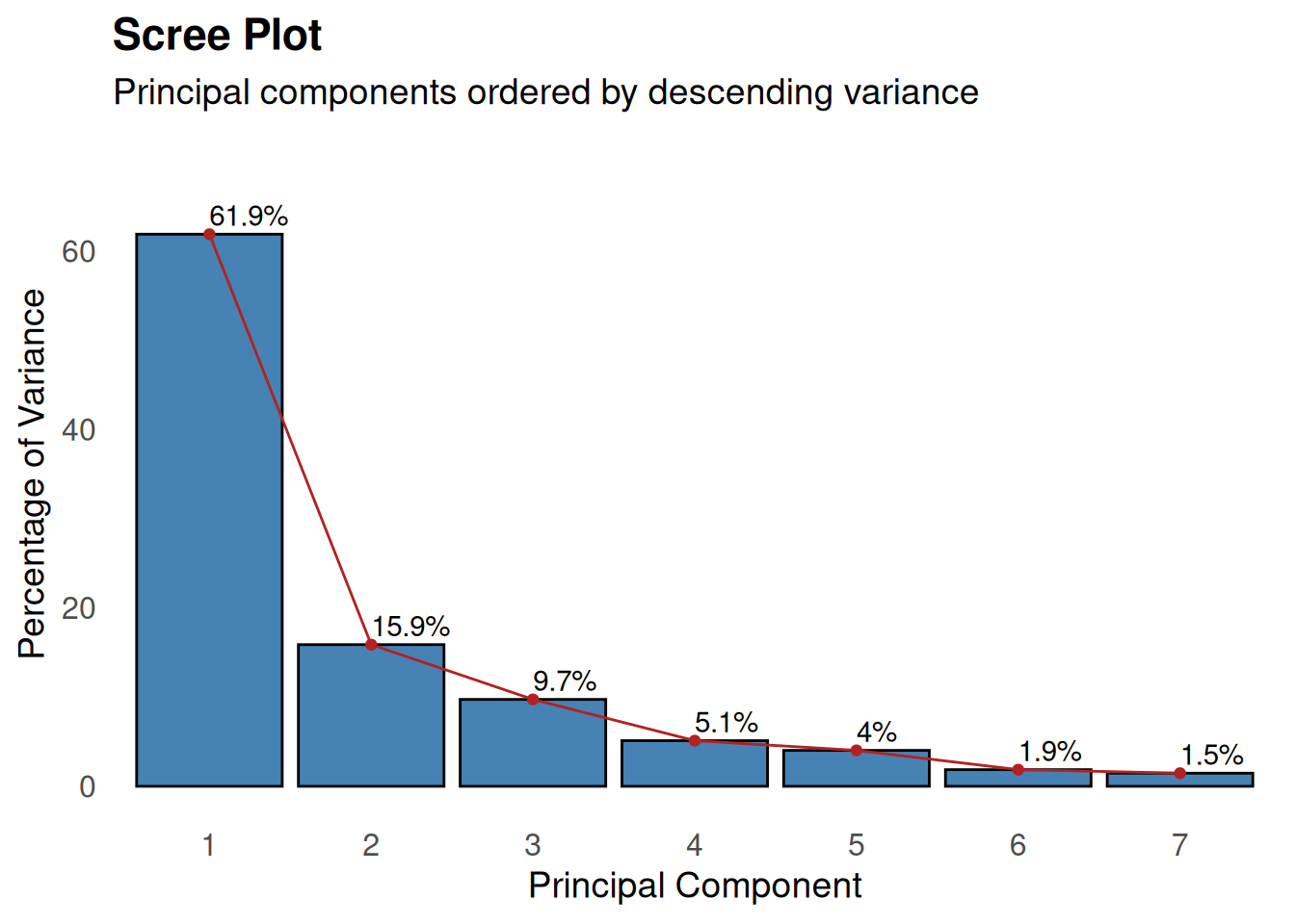

# PCA biplot
fviz_pca_biplot(
  pca,
  label       = "var",              # show only variable (arrow) labels
  repel       = TRUE,               # avoid text overlap
  geom.ind    = "point",            # draw points for observations
  pointshape  = 21,
  pointsize   = 2.5,
  alpha.ind   = 0.3,    
  fill.ind    = data$gender,        # use your gender factor
  col.ind     = "black",            # point border
  palette     = c("salmon", "skyblue"),
  col.var     = "black",        # arrow color
  col.var.dim = 1,                  # arrow color by dimension?
  addEllipses = TRUE,               # concentration ellipses by group
  ellipse.level= 0.68,              # 68% confidence ellipse
  legend.title = list(fill = "Gender")
) +
  labs(
    title = "PCA Biplot",
    subtitle = "Observations colored by Gender; Variables as arrows"
  ) +
  theme_minimal(base_size = 14) +
  theme(
    plot.title    = element_text(face = "bold"),
    plot.subtitle = element_text(color = "gray40"),
    legend.position = "right"
  )